Testing Malus's law with Arduino

An experiment with polarized light, a LEGO apparatus, and an Arduino light sensor-and what I learned when the measurements did not match the expected curve.

In my fifth year of high school, I investigated Malus’s law: how the intensity of polarized light changes as we rotate a polarizing filter. I built an apparatus using LEGO, a laser diode, two polarizers, a photoresistor, and an Arduino Uno. The experiment brought together the physics of light and the electronics needed to measure it.

The most interesting part came when the first results did not follow the curve I expected. I had to look beyond the optical setup and question how I was converting the sensor readings into light intensity. Here, I’ll walk through the experiment, the original measurements, and the limits of the interpretation I used at the time.

Information:

You can download all 65 readings as a CSV, with column definitions and calculation notes. The interactive charts below use my experimental data. Hover or tap a point for its voltage and resistance, drag to zoom, and click a legend entry to hide or show a series. Double-click the plot to reset its view; a static chart is available below each plot.

1. What we expect from two polarizers

A linearly polarized light wave has an electric field that oscillates along a fixed direction perpendicular to the direction of propagation.

An ideal linear polarizer transmits the electric-field component parallel to its transmission axis. If the incident field has amplitude \(E_0\) and makes an angle \(\theta\) with that axis, the transmitted amplitude is

\[E = E_0\cos\theta.\]

Because intensity is proportional to the square of the field amplitude, we obtain Malus’s law:

\[I(\theta)=I_0\cos^2\theta.\]

Here, \(I_0\) is the intensity of the linearly polarized beam immediately before the analyzer, which is the second polarizer in my apparatus. The angle \(\theta\) is measured between the transmission axes of the two filters. For the ideal case, parallel axes transmit the maximum, crossed axes transmit no light, and a 45° angle gives half the maximum. This is the projection argument described in OpenStax’s explanation of polarization.

Relative angle	Ideal transmitted fraction
0°	100%
30°	75%
45°	50%
60°	25%
90°	0%
180°	100%

I suggest keeping the distinction between field amplitude and intensity in mind: the projection gives a cosine, while the intensity follows its square. The pattern repeats every 180°, since reversing a filter’s axis gives the same transmission direction.

2. Building the apparatus

My optical path was straightforward:

Laser → fixed polarizer → rotating analyzer → photoresistor.

The first polarizer established a fixed polarization direction, while the second let me vary the angle without rotating the laser itself. The laser pointed downward through the filters toward the sensor. I used a white LEGO support to hold the components and allow manual adjustment of their alignment. The presentation also describes an opaque cardboard enclosure around the structure to reduce interference from room light. The detector was an LDR, or light-dependent resistor: its resistance decreases as more light reaches it. The Arduino measured the voltage across it in a voltage divider, then sent the readings over USB serial. My report describes averaging multiple readings for each measurement and switching the laser on only during acquisition to limit heating. The exact number of samples and acquisition timing are not recorded in the supplied report, so I cannot reconstruct those details here. For each main measurement set, I recorded 13 angles in 15° steps, covering a half-turn. The report assigns an angular uncertainty of approximately ±2°, based on the markings and manual positioning of the filters.

3. From Arduino voltage to resistance

The circuit used a nominal 5 V supply and a 100 kΩ fixed resistor in series with the LDR. The fixed-resistor value appears in both the presentation’s circuit diagram and the spreadsheet formulas. The voltage was measured across the LDR, rather than across the fixed resistor.

Voltage-divider circuit with a 5 V supply, a 100 kiloohm fixed resistor, and voltage measured across the photoresistor. — The circuit diagram from my original presentation; the 10 kΩ label beside the LDR illustrates a resistance value, rather than a second fixed resistor.

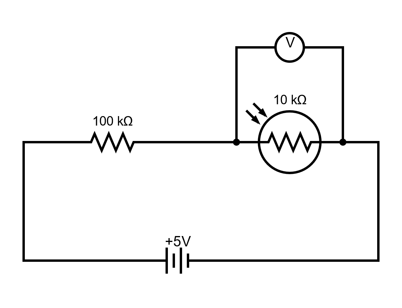
Calling the measured voltage \(V\), the supply \(V_s\), and the fixed resistance \(R_f\), the divider gives

\[V=V_s\frac{R_{\mathrm{LDR}}}{R_f+R_{\mathrm{LDR}}}.\]

Solving for the sensor resistance gives

\[R_{\mathrm{LDR}}=R_f\frac{V}{V_s-V}.\]

For example, the first set’s reading at 0° was 0.4494 V. Using the nominal circuit values, we obtain

\[R_{\mathrm{LDR}}=100\,\mathrm{k\Omega}\times\frac{0.4494}{5-0.4494} \approx9.8756\,\mathrm{k\Omega}.\]

The direction of the response can seem surprising at first: more light lowers the LDR resistance, which also lowers the voltage measured across it. We therefore cannot treat the voltage itself as a quantity proportional to light intensity.

4. Checking the laser before testing the law

Before interpreting the two-filter measurements, I rotated a single filter relative to the stationary laser and support. The detected signal changed with orientation. In my original report, I interpreted this as evidence that the laser beam was partially polarized.

Single-filter control: normalized inverse resistance, used as a detector proxy.

This chart uses normalized inverse resistance as a sensor proxy, rather than a calibrated intensity measurement. Its vertical axis starts at 75% to make the variation visible. The control suggested that I should not assume the incident beam was unpolarized, although it did not independently determine its degree of polarization. Alignment changes could also affect such a measurement.

Keeping the first polarizer fixed gave the main experiment a defined input polarization while I rotated only the analyzer. The familiar statement that a polarizer transmits half the incident intensity applies to ideal, unpolarized incident light; it should not be assumed for this laser. For the angular comparison, I instead worked with relative signals.

5. The first conversion did not reproduce the expected curve

My initial analysis assumed a simple inverse relationship between resistance and light level \(L\):

\[R=\frac{k}{L}.\]

If that model were adequate, an unknown constant \(k\) would cancel when taking a ratio:

\[\frac{L}{L_{\mathrm{ref}}}=\frac{R_{\mathrm{ref}}}{R}.\]

The report initially used a reference measurement with only the fixed polarizer in place. For Set 1, that reference was 0.4492 V, corresponding to approximately 9.8708 kΩ. The workbook also normalized each two-filter sweep to its own inferred maximum, using the minimum resistance in that sweep. I use this second convention consistently in the comparison charts:

\[y_{\mathrm{inverse}}=\frac{R_{\min}}{R}.\]

This normalization makes the maximum equal to one, but it does not establish an absolute light calibration or measure the analyzer’s insertion loss. The first sweep shows why that distinction matters.

Angle	Measured voltage (V)	Derived resistance (kΩ)	Inverse-model ratio	Ideal \(\cos^2\theta\)
−45°	0.4950	10.9878	0.8988	0.5000
0°	0.4494	9.8756	1.0000	1.0000
30°	0.5097	11.3511	0.8700	0.7500
45°	0.5535	12.4480	0.7934	0.5000
60°	0.6676	15.4095	0.6409	0.2500
90°	4.0088	404.4391	0.0244	0.0000

At 45°, this conversion suggests roughly 79% of the maximum, whereas the ideal prediction is 50%. The differences are too large to describe as a close quantitative match. The readings at −45° and +45° also differ, even though the ideal curve is symmetric. A sensor conversion alone cannot explain every feature of the data.

6. Trying a different sensor model

I then explored an empirical exponential conversion:

\[L=\alpha e^{-\beta R}.\]

Normalizing to the same sweep’s maximum removes \(\alpha\):

\[y_{\mathrm{exponential}}=\frac{L}{L_{\max}} =e^{\beta(R_{\min}-R)}.\]

The workbook uses \(\beta=0.47\,\mathrm{k\Omega}^{-1}\) for Sets 1, 2, and 3. When resistance is expressed in ohms, the equivalent value is \(4.7\times10^{-4}\,\mathrm{\Omega}^{-1}\). The units must match so that the exponent is dimensionless.

Set 1: the same voltage readings converted using two sensor models, with ±2° horizontal error bars.

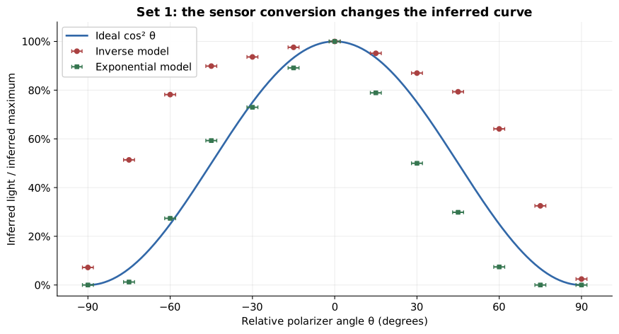
The red points use the original inverse model, while the green points use the exponential model. The blue line is the ideal prediction, and the horizontal bars show the report’s ±2° angular uncertainty. Both sets of points come from the same measured voltages. The curve changes because the conversion changes, rather than because I collected a new set of readings.

The exponential model brings many points closer to the expected shape, but substantial discrepancies remain. For example, the converted values at −45° and +45° are approximately 0.593 and 0.298, compared with a theoretical value of 0.5 for both. I would describe this as improved agreement under an empirical model, rather than a precise verification of the law.

An LDR is not automatically a calibrated light meter. Its response depends on the particular sensor and the illumination conditions, as discussed in Adafruit’s photocell guide. The exponential expression here was an exploratory approximation from my original project, not a universal law for photoresistors.

7. Repeated measurements and Set 4

The workbook contains two further sweeps analyzed with the same value of \(\beta\). They cover 0° to 180°, rather than the −90° to +90° interval used in Set 1.

Sets 2 and 3: both sensor conversions compared with the ideal curve, retaining all readings.

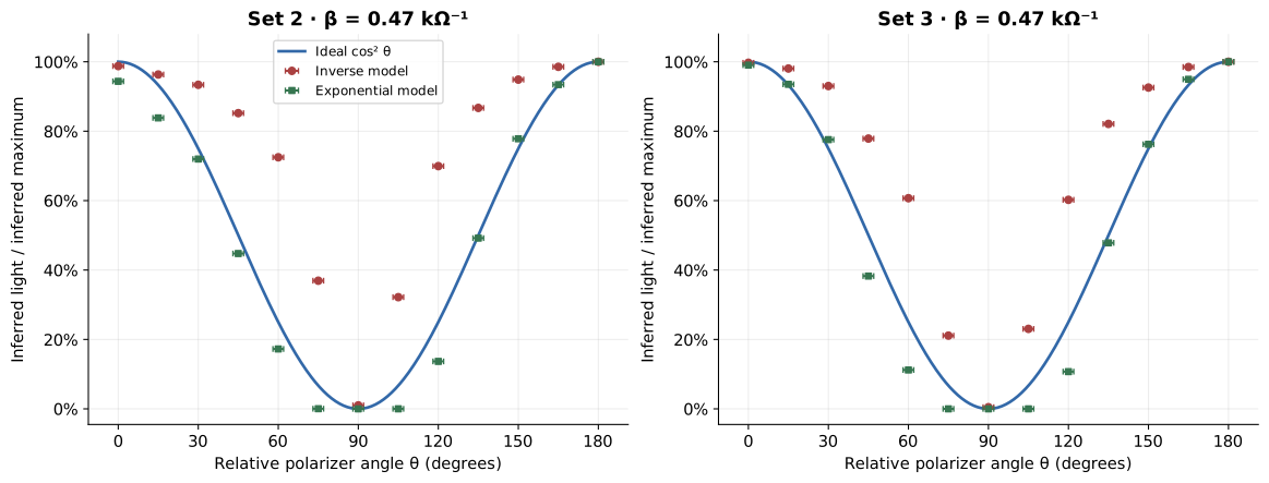
A fourth measurement set records a run made under different conditions. It uses \(\beta=0.07\,\mathrm{k\Omega}^{-1}\), rather than 0.47. The spreadsheet notes better shielding from ambient light and warmer, more humid conditions as possible reasons for differences between runs; these were proposed explanations, rather than separately measured causes. It also flags possible positioning errors in the first and last readings.

Set 4: both sensor models and all thirteen readings, including the flagged endpoints.

For this chart, I shifted Set 4’s recorded angles from 90°–270° to −90°–90° by subtracting 180°. This leaves the theoretical cosine-squared values unchanged. I kept all 13 measurements, including the two flagged endpoints.

To compare the curves numerically for this article, I recalculated the root-mean-square deviation from the ideal prediction:

\[\mathrm{RMSE}=\sqrt{\frac{1}{N}\sum_{i=1}^{N} \left(y_i-\cos^2\theta_i\right)^2}.\]

Each row below uses all 13 points, with equal weight and the workbook’s original \(\beta\) value. These are descriptive deviations in normalized units, not uncertainty estimates or formal goodness-of-fit tests.

Measurement set	Inverse-model RMSE	Exponential-model RMSE	\(\beta\) (kΩ⁻¹)
Set 1	0.278	0.116	0.47
Set 2	0.266	0.058	0.47
Set 3	0.205	0.070	0.47
Set 4	0.058	0.056	0.07

The exponential conversion reduces the deviation in the first three sets, while Set 4 shows only a small difference between the two conversions. The change in \(\beta\) is also a reason to avoid treating it as a transferable sensor calibration.

8. What the experiment could establish

The experiment showed a repeatable dependence of the detected signal on the relative orientation of the polarizers. Its broad pattern is consistent with the expected transmission maximum for aligned filters and minimum for crossed filters. It also exposed how strongly an inferred intensity curve can depend on the detector model.

There is an important limit to the calibration argument: I selected an empirical conversion because it made the data resemble the law I wanted to test. That agreement cannot independently validate both Malus’s law and the sensor conversion. An independent calibration would be needed to separate those questions.

The source material does not provide repeated-reading scatter, a complete voltage uncertainty budget, or an independently measured light-to-resistance calibration. For that reason, I have not added vertical error bars or claimed agreement within experimental uncertainty. The recorded decimal places describe the stored readings, rather than establishing their accuracy.

The divider also becomes sensitive to voltage error as its reading approaches the supply:

\[\frac{dR}{dV}=R_f\frac{V_s}{(V_s-V)^2}.\]

That matters near crossed polarizers, where a high LDR resistance pushes the measured voltage toward 5 V. Background light, imperfect extinction, alignment, sensor response time, and heating are further effects I would investigate before assigning a discrepancy to the optical law.

If I repeated the project, I would first calibrate the detector independently, record dark readings, repeat each angle, and measure the supply voltage. I would also compare the result with a photodiode operated in a characterized linear regime. Those changes would make the comparison less dependent on choosing a convenient conversion afterward.

Experimental data

I have provided a CSV containing all 65 readings and the derived quantities used here, with column definitions and calculation notes. It includes the laser control and Sets 1–4. The CSV and charts are a new extraction of the original workbook; the RMSE comparison is an additional calculation for this article.

Looking back, the most useful lesson was learning to question the measurement chain. The Arduino supplied voltages, the circuit let me derive resistances, and only a further model turned those resistances into relative light levels. Understanding each of those steps was as much a part of the experiment as rotating the polarizers.

Enjoyed reading this article?

Here are some more articles you might like to read next: